Create an Excel lookup formula that searches a table using criteria from various columns. It mimics the functionality of the native VLOOKUP() formula using a combination of the INDEX() and MATCH() function.
Ingredients
- Microsoft Excel
The Need
There is no doubt that one of the most useful and often used Excel functions is the VLOOKUP() function. This function allows us to extract values from a table by specifying a search criteria. However, as we start developing more complex spreadsheets and calculations, we start finding some of its limitations.
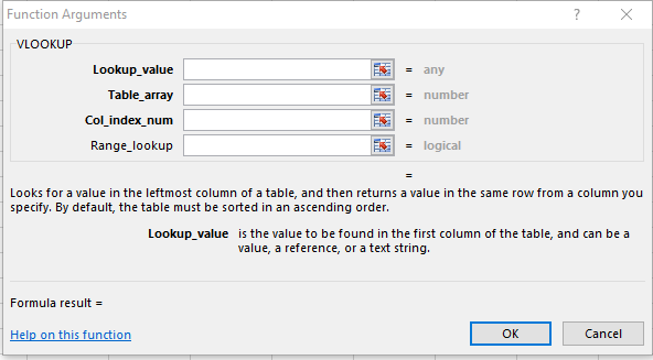
One of this limitations is the fact that the VLOOKUP() function can only search one column (the left-most) within the specified search range.
As you can see, the “Lookup_value” is searched on the “Table_array” leftmost column and only on that column. But what if we want to extract the value of a row where two or more search parameters are needed?
For example, in the following table, we would like to find the “ID” of the row that satisfies two conditions, the name of the Company AND the Job Title of the Employee.
In this scenario, we would like to enter two search parameters (Company and Job Title) and have the formula return the ID of that row.
We are going to use two elements of Excel functionality to achieve this:
- The combination of the INDEX() and MATCH() functions in a similar way to the way we used them in a previous post (Excel Lookups in any Direction)
- A way to enter ARRAY formulas in Excel.
The Recipe
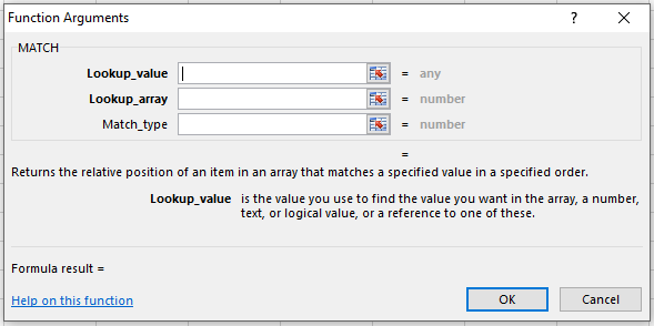
As you know, the MATCH() function will lookup a given search value within an array and return the position of the found value within the array. This is the most common use for the MATCH() function.
We’re going to use the MATCH function in a less usual way, enter ARRAY formulas.
Most of the time we use formulas (functions) in Excel to return SINGLE values. However, another way to write formulas in EXCEL is to have them return ARRAYS. This formulas return a collection (array) of values rather than a single value.
In Excel, an ARRAY formula is entered by pressing the “CTRL + SHIFT + ENTER” keys. A way to tell that a formula has been entered as an ARRAY formula rather than a “regular” formula is by looking at the formula bar. The formula will appear between curly braces { }. See the example below.
In this example we are using this technique to have the function return the position (row number) where the criteria is met in BOTH the Company column and the Job Title column.
The trick is in the way we’re specifying the “Lookup_array” parameter of this function. Rather than selecting a range of the spreadsheet, we create a “dynamic” range. This is achieved by multiplying the results of two comparison statements.
By multiplying the two lines above, an ARRAY is returned with all elements of the array being 0 (false) and the element at the position where the statements are both true returning a 1 (true).
A way to visualise this is by inspecting the function. Look at the result shown for the “Lookup_array” element.
This element shows an ARRAY of zeros with a one (1) where the two statements are true. By entering this formula into the cell as an array formula (CTRL + SHIFT + ENTER) the cell returns the number of the row where the two conditions are met. If no row meets the conditions, the formula returns a “#N/A” error which you can easily detect.
Finally, this row number can then be used on an INDEX() function of the column that you need to retrieve the value from, in our case, the ID column.
This is a very powerful combination which can allow you to build more sophisticated search and find algorithms within your spreadsheets.
You can download the sample file here:
That’s it!. We hope you found this recipe useful. If you did, please share this post in the social network of your choosing by clicking one of the buttons below.


