Short Description
Perform searches in Excel rows or columns and extract data in any direction from the found reference.
The final form of this recipe is:
Searching a column and returning a value in another column
=INDEX(<Column to extract value from>,MATCH(<Value of criteria used for looking>,<Column to be searched for value>,0))
Searching a row and returning a value in another row
=INDEX(<Row to extract value from>,1,MATCH(<Value of criteria used for looking>,<Row to be searched for value>,0))
Ingredients
- Microsoft Excel
The Need
In many scenarios, data held in the form of a table needs to be searched for a certain criteria and when the criteria is met some piece of data has to be extracted from the table. This search for particular criteria can be done either by columns or rows. Enter the VLOOKUP and HLOOKUP functions.
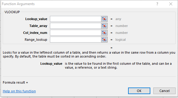
The VLOOKUP (and its sister HLOOKUP) function requires at least three parameters: “Lookup_Value”, “Table_array” and “Col_index_num”.
As the function description explains, this function:
Looks for a value (“Lookup_Value”) in the leftmost column of a table (“Table_array”), and then returns a value in the same row from a column you specify (“Col_index_num”).
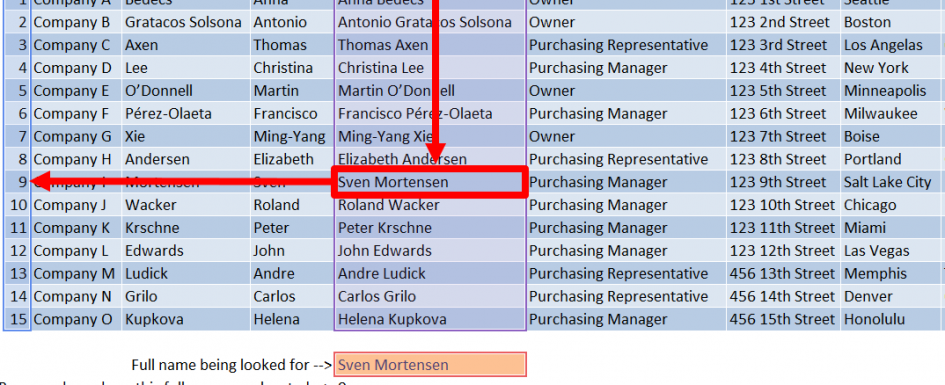
However, in many instances you might want to search for a value on a column (or a row in the case of HLOOKUP) and return a value to the LEFT of that column (or ABOVE the searched row).
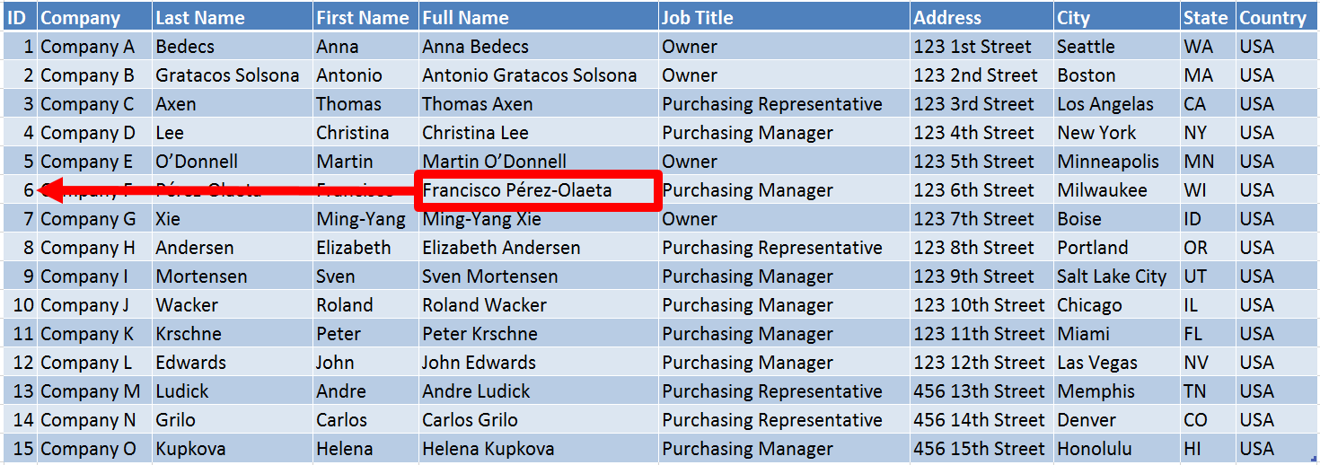
For example, in a table of “Customers” information, you might want to be able to search by the Full Name of the client and have the function return the ID of that customer.
The Recipe
The desired functionality is achieved by replacing the VLOOKUP (or HLOOKUP) function with the combination of two other functions: INDEX and MATCH.
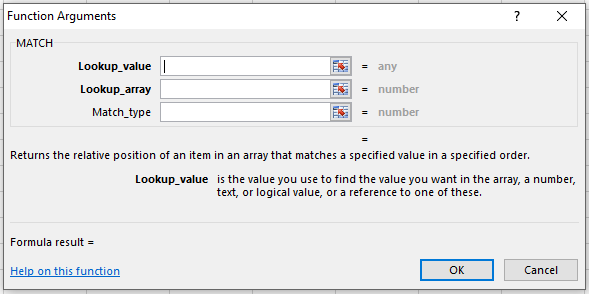
The MATCH function returns the position of a certain element within an array (“Lookup_array”) that matches the specified criteria (“Lookup_value”).
We use the MATCH function to search through a column (or row) and find the row position of the cell that matches the criteria we’re after. In our example, we are going to look for a customer’s full name, so that is our entry value and will be the “Lookup_value” argument.
For “Lookup_array” we will specify the column of the table that we want to search, in our example is the “Full Name” column.
The third (optional) parameter of this function can be used to specify whether we want an approximate or an exact match to consider the value found. In most cases you’ll want to find the exact value to avoid false positives. Enter a zero (0) to indicate this exact match choice.
The final formula looks like:
If you place the result of this formula on a cell, it will give you the row number where the full name is, in this case 9.
In the next step we will use the value obtained from the MATCH function as one of the inputs to the INDEX function. The INDEX function returns the value at a specific location within a range.
In our case, we want to extract the ID of the customer that matched the full name we entered.
The final formula, which combines the MATCH and INDEX functions in one cell, would look like this:
As seen in the screen shot above, the MATCH function searches through the [Full Name] column looking for the value entered in the cell “FullNameLookedFor”. This then is used by the INDEX function to return the value of the cell in the [ID] column moving that number of rows down.
The above combination is a powerful aid to search for values in any row or column and return values from any other row or column irrespective of their relative locations in the table.
That’s it!. We hope you found this recipe useful. If you did, please share this post in the social network of your choosing by clicking one of the buttons below.


